Artificial Neural Networks

---

Motivation

Funktionale Nachbildung eines Neurons

---

Forward pass

$$out = f(b + \sum_i {x_i \cdot w_i}) = f(b + \textbf{x}\textbf{w}^T)$$

• $x_i\dots$ Inputfeatures

• $w_i\dots$ Weights, Parameter

• $b\dots$ Bias

• $f\dots$ Aktivierungsfunktion

---

Network

---

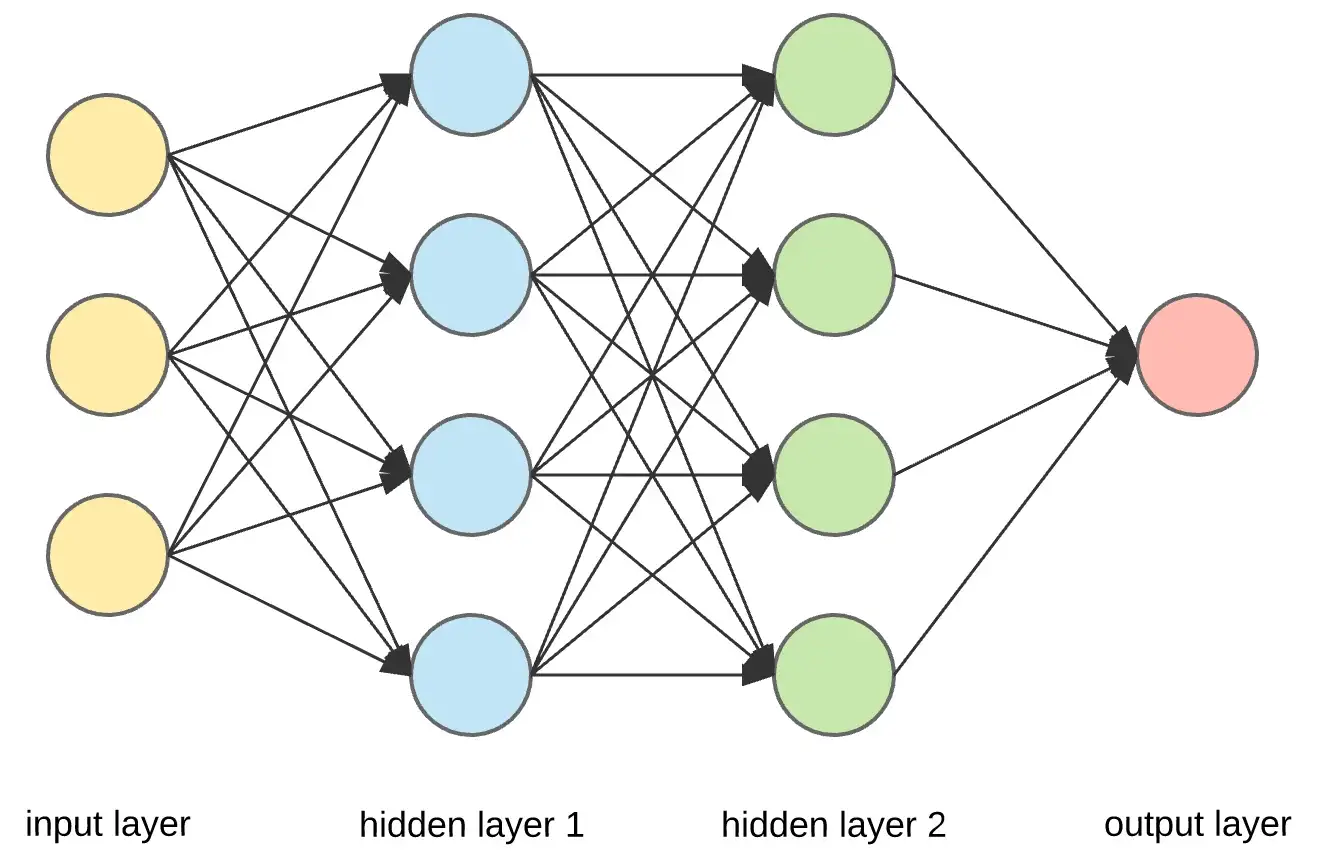
$$\textbf{out}_1 = f(\textbf{x}\cdot\textbf{W}_1)$$

$$\textbf{out}_2 = f(\textbf{out}_1\cdot\textbf{W}_2)$$

$$\textbf{y} = f(\textbf{out}_2\cdot\textbf{W}_3)$$

$$\textbf{y} = f(f(f(\textbf{x}\cdot\textbf{W}_1)\cdot\textbf{W}_2)\cdot\textbf{W}_3)$$

---

Aktivierungsfunktion

$$f_1(x) = k_1x + d_1, f_2(x) = k_2x + d_2$$

$$f_1(f_2(x)) = k_1f_2(x) + d_1 = k_1(k_2x + d_2) + d_1$$

$$f_1(f_2(x)) = k_1k_2x + k_1d_2 + d_1$$

$$f_1(f_2(x)) = \underbrace{k_1k_2}\textrm{k}x + \underbrace{k_1d_2 + d_1}\textrm{d}$$

Ohne Aktivierungsfunktionen nur lineare Zusammenhänge

---

---

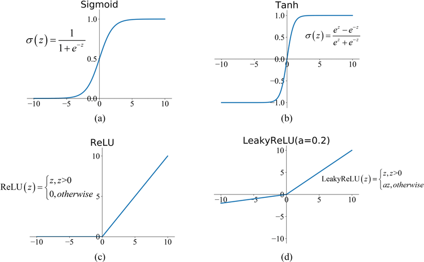
Auswahl

• Hidden Layer: *elu
• Output layer

  Regression

  Keine $\rightarrow y=x$

  Loss: MSELoss()

---

Klassifikation

Logits ⟹ Probabilities ⟹ Classes

Binäre Klassifikation

Sigmoid() / BCELoss()

keine / BCEWithLogitsLoss()

Linear(in_features=42, out_features=2)
Softmax(dim=1)
      

Multi-class-classification

keine / CrossEntropyLoss()

Softmax() / CrossEntropyLoss()

Linear(in_features=42, out_features=class_count)
Softmax(dim=1)
      

---

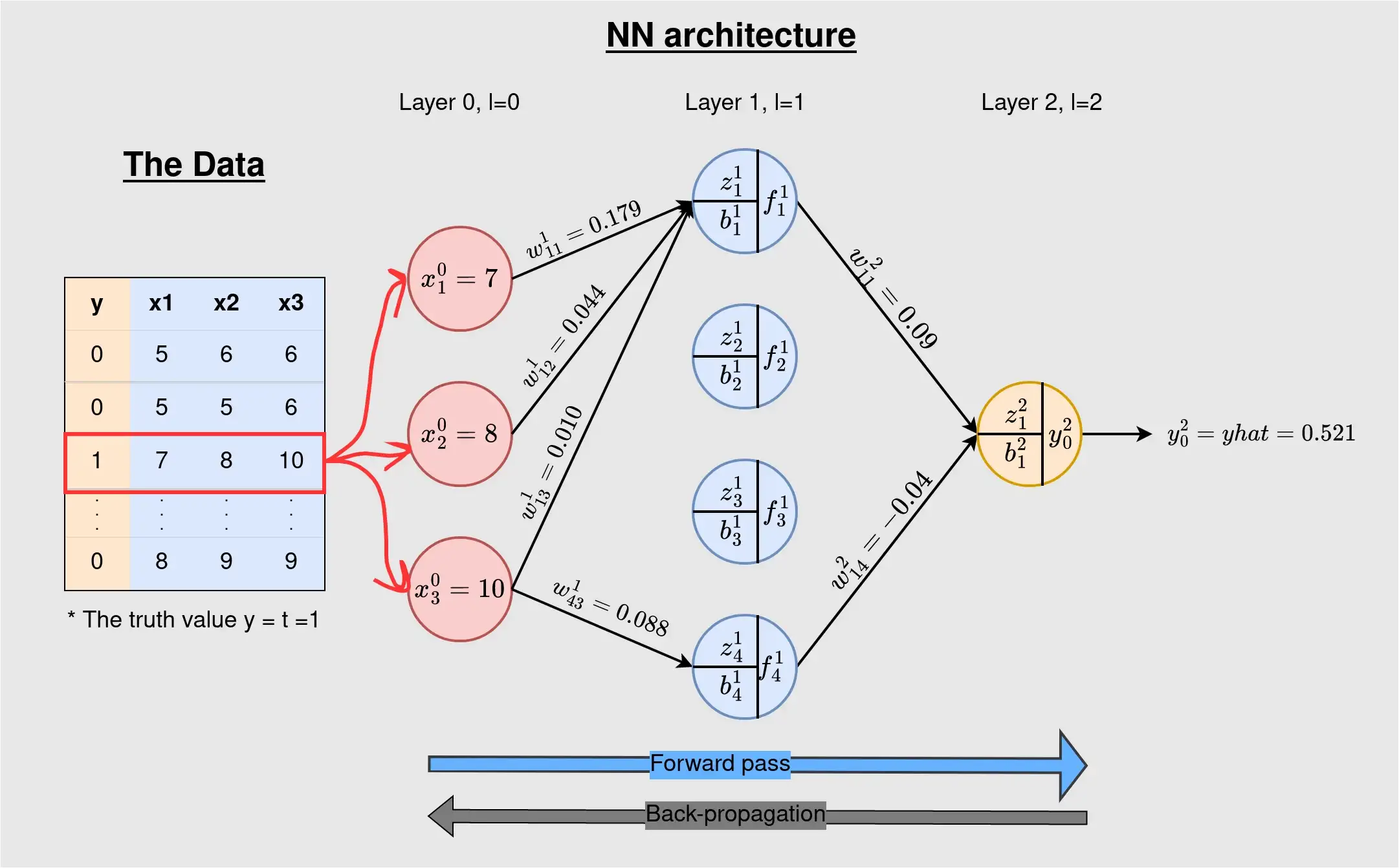
Training

1. Alle $w_i$ random initialisieren

2. forward pass:
   Observation -> Output

3. Loss $L(y_{true}, y_{pred})$ berechnen

4. backward pass/backpropagation:
   $w_i$ anpassen vom output-Layer bis zum input-Layer

for X, y in data:
  prediction = model(X)
  error = loss_fn(y, prediction)
  update_weights(error, loss)

---

Forward pass

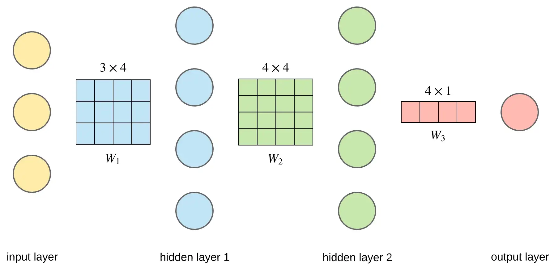
$$ 1 \times 3 \cdot 3 \times 4 = 1 \times 4$$

---

---

Backward pass

• $L(y_{true}, y_{pred}),\qquad y_{pred}(\textbf{x}, \textbf{w})$

• $\implies L(y_{true}, \textbf{x}, \textbf{w})$

• $\implies$ Anpassen der weights $\textbf{w}$, sodass Fehler $L$ minimal

---

Gradient Descent

---

---

Learning rate

---

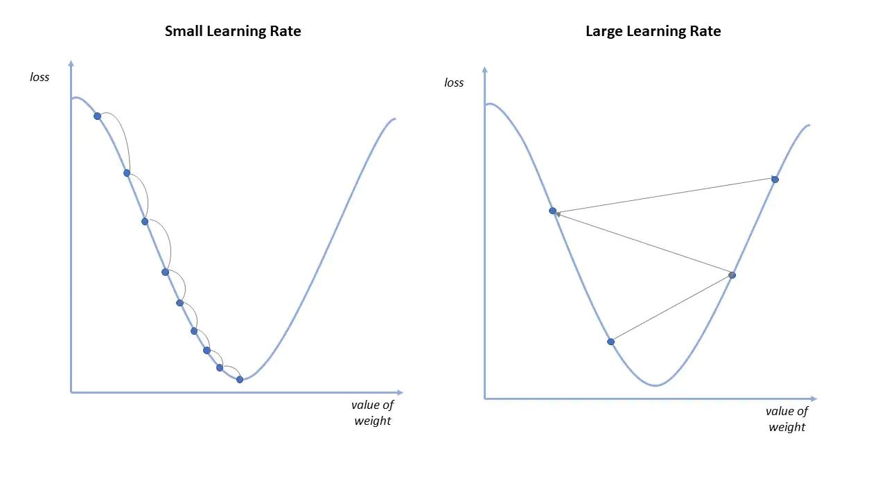
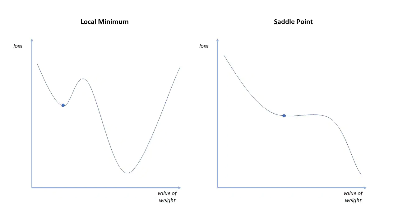
Probleme

---

Momentum

---

Backpropagation

$$w_{t+1} = w_t - \eta\frac{\partial L}{\partial w_t}$$ $\eta\dots $ learning rate

---

Kettenregel

$$y = f(u), u = g(x)) \implies y=f(g(x))$$

$$\implies y' = f(g(x))'= f'(g) \cdot g'(x)$$

$$y = sin(x^2) \implies y' = cos(x^2) \cdot 2x$$

$$\frac{dy}{dx} = \frac{dy}{du}\frac{du}{dx}$$

---

---

$$\frac{\partial L}{\partial w^2_{11}} = \frac{\partial L}{\partial \hat{y}} \frac{\partial \hat{y}}{\partial z_1^2} \frac{\partial z_1^2}{\partial w^2_{11}}$$

\begin{align} \frac{\partial z_1^2}{\partial w^2_{11}} = &\frac{\partial}{\partial w^2_{11}}(f_1^1 w^2_{11} + f_2^1 w^2_{12} + f_3^1 w^2_{13} + f_4^1 w^2_{14} + b_1^2)\\ = &f_1^1 \end{align}

$\hat{y}(z) = \frac{1}{1+e^{-z}}$ aka sigmoid, $\hat{y}(z)' = \dots$

$$\frac{\partial L}{\partial w^2_{11}} = -0.405$$

---

Adam - Adaptive Moment Estimation

optimizer = Adam(model.parameters(), lr=1e-3)

• für jedes $w$ werden die letzten Änderungen ausgewertet

• und diese in die Backpropagation einbezogen

---

batch_size

Bei jeder observation weights updaten problematisch:

• viel Aufwand

• ständig auf/ab

• 💡 ein paar processen, Fehler mitteln

for X, y in data:
  # X.shape[0] = batch_size
  predictions = model(X) # shape = (batch_size, 1)
  error = loss_fn(y, prediction) # shape = (batch_size, 1)
  total_error = error.sum() # shape = (1, 1)
  optimizer.update_weights()